There is a particular kind of hubris that shows up in engineering projects. It is the moment you look at 87 Fortran files representing forty years of accumulated ocean physics and think: I can do this in Python. Not translate the interface. Not wrap the binary. Rewrite it. Subroutine by subroutine, comment by comment, constant by constant, until what you have is a Python package that produces the same numbers — to a scientifically meaningful degree of precision — as a compiled Fortran model that has been validated against field observations across four decades.
This is my story of pyGOTM. It is not a clean success story. It is a story of a wrong bet made confidently, a painful pivot, weeks of debugging failures that looked like successes, and a methodology I invented out of necessity when the obvious approach turned out to be wrong. It is, in the end, a story about what it means to be stubborn in the right direction.
What GOTM Is, and Why It Matters
The General Ocean Turbulence Model — GOTM — is one of the foundational tools of physical oceanography and limnology. First published in the late 1990s by Burchard, Bolding, and Villarreal, it implements one-dimensional vertical ocean physics: it takes a water column, applies atmospheric forcing at the top, resolves turbulent mixing through multiple closure schemes, and tells you how temperature, salinity, and velocity evolve over time at every depth.
“One-dimensional” sounds deceptively simple. In practice, GOTM implements nearly a dozen turbulence closure models — k-epsilon, k-omega, the Generic Length Scale formulation, Mellor-Yamada 2.5, KPP — along with complete surface flux physics (COARE bulk fluxes from Fairall et al., Kondo 1975), solar radiation absorption via Jerlov water types, ice thermodynamics, biogeochemical coupling through the Framework for Aquatic Biogeochemistry (FABM), Stokes drift, and seagrass and sediment parameterizations. The production model is roughly 87 Fortran source files. It is used by scientists worldwide for ocean mixing research, lake stratification studies, aquaculture site assessment, and water quality management.
The problem is the barrier to entry. GOTM requires a Fortran compiler, a specific build toolchain, and enough familiarity with Fortran 90 module systems to configure and run it. For oceanographers who live in Python — increasingly, most of them — GOTM is an island that requires a boat to reach.
That was my challenge.
The Vision
My goal for pyGOTM was ambitious: translate all 87 Fortran files into Python, one-to-one, preserving the directory structure, the Fortran comments as docstrings, the exact array indexing conventions (DIMENSION(0:nlev) in Fortran becomes shape (nlev+1,) in Python), and the scientific integrity of every algorithm. Make it installable from conda. Make it run in the browser eventually. And since a 1D model’s real power comes from running thousands of independent water columns simultaneously — for ensemble forecasting, for spatial surveys, for aquaculture site optimization across a whole fjord — make it fast enough to handle that load without a Fortran compiler in sight.
Above all, make it a genuine open-source contribution — a bridge between forty years of validated ocean physics and the Python ecosystem where the next generation of oceanographers already works. The turbulence closures, the air-sea flux schemes, the ice thermodynamics: all of it too carefully built over too many decades to stay locked behind a compiler and a build toolchain that fewer and fewer working scientists maintain.
The GPU angle was my first wrong turn.
The Fog Before the Code
The first commit did not happen on the first day. It happened four weeks in.
Those four weeks had no clean shape. They were the disorienting, unglamorous process of a nuclear engineer trying to understand whether he could actually do this — not the coding, but the physics. Whether a background built entirely around reactor coolant channels, thermal-hydraulic transients, and critical heat flux margins could transfer to a one-dimensional ocean water column driven by solar forcing, wind stress, and forty years of limnological literature I had never opened.
I knew turbulence. K-epsilon, k-omega, wall functions — these were the daily vocabulary of my work in nuclear thermal-hydraulics. The Reynolds-averaged equations governing a reactor coolant flow and the equations governing an ocean mixed layer are not different equations. They are the same equations, differently parameterized, differently forced, differently validated. That was my footing. Not much, but something.
What I did not know was the phenomenology: the seasonal thermocline, the diurnal mixed layer, the Monin-Obukhov surface similarity, the way a freshwater lake stratifies in summer and overturns in autumn. I had read none of it. So I read. I worked through the GOTM manual. I read through the FORTRAN source code to develop an understanding sufficient for the purpose I was aiming for.
The question I kept returning to was not “how do I translate this?” It was sharper and more unsettling: will I know if it’s wrong? A translation that produces plausible-looking numbers but contains a subtle sign convention error is not a translation — it is the wrong physics, rendered confidently. For a nuclear engineer, that kind of error has a specific name: a non-conservative assumption. The kind that passes a review and fails a validation.
Four weeks in, I believed I understood enough to begin. That belief, as it turned out, was partly right and partly wrong in exactly the ways that mattered.
The First Bet: Taichi
Four weeks into the project, the first commit landed: a Taichi-based implementation.
Taichi is a Python-embedded parallel programming language designed for physics simulation. It compiles Python-syntax kernels to GPU (and CPU) code, handles array allocation through its own field system, and offers a clean GPU-parallel pattern: an outer loop over spatial cells runs in parallel across GPU threads, while the inner serial computation handles the cell’s local physics.
The appeal was obvious. GOTM’s multi-column use case maps naturally to GPU parallelism: each water column is independent; run all of them simultaneously on GPU threads. The Taichi pattern would look like:
@ti.kernel
def step_uequation(n_cols: ti.i32, nlev: ti.i32, dt: ti.f64):
    for col in range(n_cols):    # parallel — GPU threads
        for k in range(1, nlev): # serial — Thomas algorithm
            ...
The infrastructure came together: TaichiFieldCollection base classes, ColumnLayout field allocators, TemplateArg and NdarrayArg type wrappers for strict mypy compatibility, session-scoped ti.init() fixtures for the test suite. A translation map took shape: 87 Fortran files, 87 Python files, same directory structure. The implementation plan was written in careful phases.
Phase 0 (infrastructure) passed. Phase 1 (utilities) started. Tests ran. The physics was translating.
Then Taichi broke things.
When the Foundation Crumbles
The problems accumulated quietly at first, then all at once.
Problem one: annotations. Taichi evaluates Python type annotations at decoration time to infer kernel types. That means from __future__ import annotations — a common Python 3.10+ idiom that defers annotation evaluation for cleaner syntax — is forbidden in any file that contains @ti.kernel or @ti.func. This is not documented prominently. I discovered it when a kernel silently failed to compile, then crashed with an opaque type-inference error. I had to discover the constraint, document it, and enforce it as a project rule — applied to every future physics file.
Problem two: kernel return types. Taichi 1.7.4 on Python 3.13 does not accept -> None on @ti.kernel functions — void kernels must simply omit the return annotation. This is a stack-specific quirk that differs from standard Python convention and from every other Taichi documentation example written for an earlier Python version.
Problem three: test contamination. ti.init() ran in each test fixture and ti.reset() in teardown. Taichi has a single global runtime state per process. When one test initializes Taichi with one configuration and another test resets it, subsequent tests may run with a stale or mis-configured runtime — passing in isolation, failing under pytest full-suite. The fix (a session-scoped autouse fixture) worked, but every existing test had to be updated, and the fragility was real.
Problem four: typing. Strict mypy — which the project required — could not reconcile Taichi’s ti.template() field arguments with standard Python annotations. A local typing bridge — TemplateArg, NdarrayArg, ti_kernel — papered over the gap, but it was boilerplate that added noise to every kernel definition.
Problem five: two physics paths. Early in the implementation, some modules ended up with both a plain-NumPy reference implementation and a Taichi kernel. This “dual-path” pattern was a maintenance trap: a bug shared by both would pass tests undetected, and the two paths inevitably drifted. I decided to remove the NumPy paths and commit to Taichi-only. But ripping them out required rewriting all the affected tests.
Problem six: the architecture mismatch. The deeper issue was that Taichi’s model — GPU threads over a flat field of work — does not map cleanly to GOTM’s vertical solvers. The Thomas algorithm at the heart of GOTM’s implicit diffusion and momentum equations is inherently serial: each level depends on the previous one. You can parallelize across columns (the outer loop), but not within a column. Taichi’s GPU model excels at embarrassingly parallel workloads; I was asking it to accelerate a fundamentally serial inner loop parallelized across many independent instances.
One day after the first commit, the Taichi-to-Numba migration plan was written.
The Hard Decision
There is a specific kind of pain in walking away from something you have already built. The Taichi implementation worked. Tests passed. Physics translated correctly. The architecture was documented, the patterns were established.
But the constraints were accumulating faster than the physics was. Every new file would need the same annotation workaround, the same -> None omission, the same mypy bridge. The GPU deployment model was over-engineered for a model that needed, most urgently, to run correctly on CPU with eventual parallelism.
I wrote the migration plan clearly and without sentimentality:
Taichi is completely removed. No
import taichimay exist anywhere insrc/ortests/after this migration.taichiis removed frompyproject.toml.src/pygotm/fields.pyandsrc/pygotm/taichi_typing.pyare deleted. Every Taichi construct is replaced with a Numba or plain NumPy equivalent. The module structure, public API signatures, algorithm logic, and validation criteria are all unchanged. Only the acceleration layer changes.
That last sentence was crucial. Not a rewrite. A layer swap.
Soon after, I committed (literally and figuratively ) to the Numba-optimized architecture.
A Different Parallelism Philosophy
Numba’s model suited GOTM better in every way that mattered.
The physics kernels became @numba.njit(cache=True) functions — JIT-compiled to native machine code at first call, cached to disk so subsequent runs are warm. The workspace pattern became simple Python classes holding plain NumPy arrays, with no base class needed:
class TridiagonalWorkspace:
    def __init__(self, nlev: int) -> None:
        shape = (nlev + 1,)
        self.au = np.zeros(shape, dtype=np.float64)
        self.bu = np.zeros(shape, dtype=np.float64)
        self.cu = np.zeros(shape, dtype=np.float64)
        self.du = np.zeros(shape, dtype=np.float64)
        self.ru = np.zeros(shape, dtype=np.float64)
        self.qu = np.zeros(shape, dtype=np.float64)
No field allocation system. No GPU runtime. No annotation constraints. Just NumPy arrays, passed explicitly into JIT functions, with all the Python tooling working normally.
The multi-column pattern — the original GPU dream — was preserved, but implemented at two levels. A batch kernel uses numba.prange to process multiple columns in parallel across CPU threads:
@numba.njit(parallel=True, cache=True)
def step_uequation_batch(batch_size, nlev, dt, u, nu_u, ...):
    for b in numba.prange(batch_size):   # parallel — CPU threads
        step_uequation(nlev, dt, u[b], nu_u[b], ...)  # serial vertical physics
That is the inner level: kernels that can process a batch of independent columns with numba.prange while keeping each vertical solve serial. The outer level is Dask, used in the current implementation at the level where it is most robust: independent cases.
For validation, pyGOTM has built-in Dask orchestration. The serial command is:
conda run -n pygotm python -m pygotm.validation.run_validation \
    --cases couette,channel,entrainment
Adding workers switches the runner from the serial loop to a local Dask cluster:
conda run -n pygotm python -m pygotm.validation.run_validation \
    --all --workers 4 --dashboard-port 8787
The implementation is intentionally simple. If there is only one case, or if --workers is 1, run_validation.py loops in-process. If --workers is greater than one and more than one case is selected, it calls run_cases_parallel. That function creates a dask.distributed.LocalCluster with threads_per_worker=1, processes=True, and the worker count clamped to the number of selected cases. It then submits one validation case per Dask future. Each worker runs the same single-case path: resolve the reference case, run pyGOTM unless --no-run is set, compare the generated NetCDF against the Fortran reference NetCDF, and write that case’s HTML report. The parent process receives completed futures as they finish, prints progress, restores the original case order, and writes the final validation/report.html, validation/report.json, and validation/results.json.
That validation path still requires the external GOTM reference-data tree under validation/reference/. Dask does not remove that requirement; it just lets several official reference cases run at the same time.
For non-validation work — the real “run a thousand fjord sites” use case — the pattern is different. There is no special validation runner involved, and no Fortran reference data is needed. Each task is just a normal pyGOTM run from a YAML configuration:
from pathlib import Path

from dask import delayed, compute
from dask.distributed import Client, LocalCluster

from pygotm.driver import GotmDriver


def run_column(config_path: str, output_path: str) -> str:
    ds = GotmDriver(config_path).run(output_path=Path(output_path))
    ds.close()
    return output_path


configs = [
    "sites/site_001/gotm.yaml",
    "sites/site_002/gotm.yaml",
    "sites/site_003/gotm.yaml",
]

tasks = [
    delayed(run_column)(config, f"runs/{Path(config).parent.name}.nc")
    for config in configs
]

with LocalCluster(n_workers=8, threads_per_worker=1, processes=True) as cluster:
    with Client(cluster):
        outputs = compute(*tasks)
The important rule is that each task writes to its own output file. Dask is not sharing mutable model state between columns; it is launching many independent single-column simulations. On a laptop, that means local processes. On a workstation, it means more local workers. On a cluster, the same task graph can be sent to a distributed scheduler. The model code does not need to know whether it is running as one case in a validation sweep or one site in a thousand-member production ensemble.
The migration checklist was applied file by file:
[ ] Remove: import taichi as ti
[ ] Add:    import math, import numba, import numpy as np
[ ] Replace: @ti.func  →  @numba.njit(cache=True)
[ ] Replace: @ti.kernel → two functions: single-column + batch
[ ] Replace: ti.sqrt/exp/log → math.sqrt/exp/log
[ ] Replace: TaichiFieldCollection subclass → workspace class with np.ndarray attrs
[ ] Test: single-column correctness + batch parity
What Does “Correct” Even Mean?
Here is where I ran into a wall that no migration plan had anticipated.
Validating pyGOTM against Fortran GOTM sounds straightforward: run both on the same input, compare the NetCDF output. If the numbers match within some tolerance, the Python implementation is correct.
The problem is floating-point arithmetic.
Modern compilers — both gfortran and LLVM, which backs Numba — perform floating-point reassociation: they rearrange the order of operations to vectorize or pipeline better, in ways that are mathematically equivalent but produce different rounding. For GOTM’s turbulence models, this is not a minor concern. The mixing equations are nonlinear and coupled: temperature drives stratification, which drives turbulence, which drives mixing, which drives temperature. Small per-timestep differences compound. In short, strongly stratified simulations, Fortran and Numba can agree to machine precision for the first twenty days of simulation and then diverge sharply as floating-point differences in the turbulence closure cascade into chaotic trajectory separation.
The initial validation approach — a range-aware combined tolerance |a−b| ≤ max(1e-7 × ref_range, 1e-12) + 5e-6 × |b| — immediately produced hundreds of “failures” that were not failures in any physically meaningful sense. The velocity profiles looked identical. The temperature structures matched. But max_abs_err for a turbulence dissipation variable would fail because two trajectories had diverged in phase after day 20.
This was not wrong code. This was chaos.
I had to ask a new question: what does scientific parity actually mean for a turbulence model? Not “do the numbers agree exactly?” but “do the simulations behave the same way?” Do they stratify at the right depth? Do the mixing events occur at the right magnitude? Does the temperature profile have the right shape?
The Fréchet Breakthrough
The answer came from computational geometry.
The discrete Fréchet distance is a measure of similarity between two curves or trajectories. Where pointwise metrics (RMSE, max absolute error) ask “how far apart are corresponding points?”, Fréchet distance asks: “what is the minimum leash length needed to walk a dog along one curve while its owner walks along the other, neither allowed to backtrack?” It captures shape and sequence, not just values.
Applied to validation, it works like this: normalize each time series onto [0, 1] using robust 1st-to-99th percentile range, then compute the discrete Fréchet distance between the normalized Fortran and Python trajectories. A distance near zero means the trajectories are shape-equivalent. A distance above 0.20 means something is structurally broken.
The status bands settled on were:
| Status | Normalized Fréchet distance | Meaning |
|---|---|---|
| PASS | < 0.01 | Shape-equivalent |
| MARGINAL | 0.01–0.05 | Small shape deviation |
| DISCREPANT | 0.05–0.20 | Deterministic implementation difference |
| BROKEN | ≥ 0.20 | Severe mismatch |
This immediately reframed my failures. The stratified open-ocean cases (gotland, ows_papa) were DISCREPANT — not BROKEN — because the trajectories had the right physical behavior even when they diverged numerically after long simulations. Short-run lake cases like lago_maggiore, entrainment, and couette were solidly PASS. The validation was finally telling the truth about what was actually different, rather than flagging floating-point noise as failures.
The deprecation list was long: max_abs_err, max_rel_err, RMSE, NRMSE, mean_abs_err, the original range-aware tolerance, all per-variable rtol/atol settings. Simpler. More honest. More scientific.
FABM: The Detour That Wasn’t
My original plan had FABM biogeochemistry as Phase 11 — after the single-column driver, after multi-column scaling, after the API and UI. Post-MVP.
I moved it to week seven.
The reason was practical: several of the failing validation cases (medsea_east, medsea_west, nns_annual) involve biogeochemical tracers from FABM. Without FABM, I couldn’t even compare those cases properly — the reference NetCDF contained variables that pyGOTM simply did not produce.
The coupling architecture was a chunked interleaved loop. Rather than coupling FABM at every timestep (which would require passing Python objects into Numba kernels), pyGOTM advances the compiled hydrodynamics for a window of timesteps, stores the resulting physical state snapshots, then hands the window to pyfabm. The biological variables advance through those snapshots; light feedback from FABM’s attenuation diagnostics modifies PAR for the next physics window.
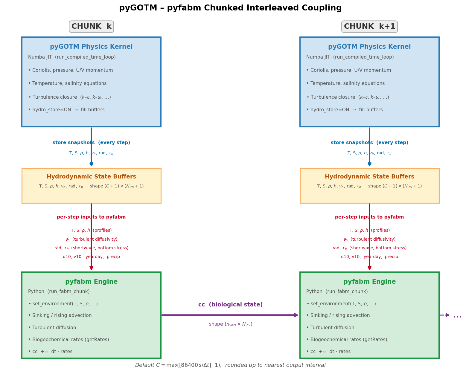
This architecture reduced trajectory divergence between FABM state and physics. It was documented carefully — the chunked approach had implications for the order of feedback terms that had to match the Fortran coupling exactly.
FABM went in cleanly, two weeks ahead of my original plan. The cases that needed it could now be compared. Some passed. Some remained DISCREPANT for biogeochemical reasons that now can be identified.
Ice and Unexpected Depth
When I paused at the eight-week mark to take stock of what I had actually built, I included a note of genuine surprise:
“Ice physics is far more comprehensive than the MVP idea suggested.”
pyGOTM ended up with five distinct ice thermodynamics models:
- No-ice limiter — the simplest path
- Simple freezing-point limiter — surface temperature clamped at freshwater or saltwater freeze point
- Lebedev FDD (Freezing Degree Day) — the canonical parameterization for freshwater lake ice, based on cumulative thermal forcing
- MyLake slab ice — the ice model used in the MyLake ecosystem model, widely used in Scandinavian lake research
- Winton three-layer sea-ice model — a more sophisticated representation with distinct snow, ice, and brine layers
- Holland-Jenkins basal melt — ocean-driven melt at the ice underside
These are not academic checkboxes. Lebedev FDD and MyLake slab ice are the standard parameterizations for cold-region freshwater reservoir modeling. Their presence in pyGOTM makes it, somewhat unexpectedly, a strong platform for winter limnology — an application I had sketched in my early roadmap but hadn’t counted on as a real technical differentiator.
The lago_maggiore validation case — a real alpine lake in northern Italy — passed Fréchet parity. A lake, correctly simulated, in Python.
The Validation Campaign
From late in week eight through week nine, my work was not physics. It was debugging.
Twenty-two official GOTM reference cases. I had to get all of them running. All of them had to produce complete NetCDF output with the correct variable schema. All of them had to be compared against the Fortran reference and produce a Fréchet report.
The failures came in several flavors:
Broken variables — variables present in the Fortran reference but absent or structurally wrong in pyGOTM’s output. These showed up as red BROKEN entries in the report. Each one meant tracing back through the NetCDF writer, the runtime buffer allocation, and the slot registration to find where a diagnostic was being omitted.
Sign convention errors — GOTM uses an “atmospheric sign convention” for surface heat flux: hflux > 0 means the ocean is losing heat (upward flux). This is the opposite of the oceanographic convention. This convention had been misapplied in the Python translation, producing temperature profiles that cooled when they should have warmed and vice versa. The error was in the translation from Fortran comments to code: the Fortran comments said “negative for heat loss” in some contexts and “atmospheric convention” in others, and the two were inconsistent with each other.
Chaotic divergence documentation — several cases (gotland, ows_papa, resolute) had deterministic divergence patterns that were reproducible but impossible to eliminate without changing the physics. The work here was to characterize them accurately, document them in docs/validation/test_cases.rst, and distinguish “this is a known floating-point behavior” from “this is a bug.”
Commit by commit, the broken variable counts came down. HTML reports were generated for each case — embedded Plotly charts showing reference and pyGOTM time series side by side for every MARGINAL and DISCREPANT variable. By the end of week nine, the suite stood at 15 PASS, 7 FAIL across 22 cases, with 2316 PASS, 67 MARGINAL, 31 DISCREPANT, and 0 BROKEN variables.
Zero broken.
Knowing What You Are
In week nine, alongside the last optimization commits, I wrote a different kind of document — an honest landscape assessment that took no prisoners.
I surveyed the ecosystem carefully: GLM-AED, FLARE, LakeEnsemblR, the long-running work at Bolding & Bruggeman ApS. Each one doing real work. Each one occupying real ground. The question I was actually asking was not “can I compete?” It was simpler and more important: what is pyGOTM for?
The answer had been there all along, in the license itself. GOTM is GPL v2. pyGOTM inherits that. The entire kernel is, non-negotiably, open-source — and that is exactly right. This was never going to be a proprietary product. It was always going to be a contribution.
What I had built was a bridge. Forty years of validated turbulence physics, re-expressed in the language the next generation of oceanographers and limnologists already uses — Python, NumPy, xarray, Numba. Scientists who (may) have never compiled Fortran, who work in Jupyter notebooks, who collaborate through GitHub: they can now run GOTM-class physics without a build toolchain, without legacy dependencies, without the steep entry cost that has kept serious ocean models out of reach for many practitioners.
Writing that down — “this is what it is, and that is enough, and it is actually important” — was not defeat. It was clarity. A working, documented, scientifically rigorous, Python-native ocean turbulence model that lowers the barrier to serious water-column physics: that is a real and valuable thing. It does not need to be a venture company to matter. The open-source community already knows how to build on something like this. I just had to finish it well enough to give it to them.
Where It Stands
Ten weeks after starting from zero — six weeks of coding after four weeks of groundwork — the pre-release cleanup went in: CI/CD workflows added, validation artifacts committed, the package cleaned for a real release.
What I built:
- A Numba-compiled Python translation of GOTM 6.0.7, 87 source files, same directory structure as the Fortran original, all Fortran comments preserved as docstrings
- 15 of 22 official GOTM reference cases passing Fréchet parity, with all 22 running to completion
- 2316 PASS, 67 MARGINAL, 31 DISCREPANT, 0 BROKEN variables in the full variable-level comparison
- Single-column wall times:
couette3.0 s,channel3.0 s,entrainment2.5 s — comparable to compiled Fortran - Five ice thermodynamics models including the lake-relevant Lebedev FDD and MyLake slab ice
- pyfabm biogeochemistry coupling with chunked interleaved architecture, bio-shading feedback, full FABM dependency supply, and metadata-discovered FABM NetCDF outputs
- COARE/Fairall and Kondo bulk flux implementations, solar/longwave radiation, Jerlov water types
- Click-based CLI:
run,validate,version,schema,cite,serve - Sphinx documentation with physics chapters on biogeochemistry, ice thermodynamics, and validation methodology
- Fréchet validation reports with embedded Plotly charts, per-variable scoring, and case-level HTML reports
- A
pygotm serveintegration surface — a warm JSON-RPC daemon for integration with other tools (like Aquirae)
The lago_maggiore alpine lake case passes. Real physics, real lake, real parity.
The full documentation covers the physics chapters, API reference, CLI usage, and validation methodology.
What Comes Next
The kernel is real. The physics is validated. My path forward is in the application layer.
Nearest on my horizon: a reservoir water-quality workflow built on the existing engine. Green Lake, Wisconsin and Falling Creek Reservoir in Virginia are my first target cases — both have excellent public datasets (USGS, EDI, WQP), published GLM-AED calibration references to compare against, and known dissolved oxygen / stratification dynamics that pyGOTM’s turbulence physics can handle directly. Dissolved oxygen, when needed, comes through FABM configuration rather than new code — the coupling is already there. Intake-depth diagnostics and basic bloom-risk indicators are post-processing on top of existing output.
The science of lake and reservoir modeling has never been more accessible in Python than it is right now. Building that accessibility was always the point.
Coda: What the Failures Taught
This is what the ten weeks actually looked like from the inside:
My first implementation was wrong. Not badly engineered — it was carefully designed, properly tested, documented. But wrong for the context.
My second implementation worked, but validating it exposed a deeper problem: I had no principled way to decide what “correct” meant for a chaotic physical system. The obvious metric (pointwise tolerance) was not the right metric.
Inventing the right metric took time and failed attempts. The Fréchet approach was not obvious. It required me to step back from the impulse to measure numerical agreement and ask what scientific parity actually means.
The FABM integration was supposed to be last. It became urgent because the problem demanded it. Plans exist to be updated.
None of that honest reckoning was wasted. Understanding what pyGOTM actually was — a bridge, not a product, a contribution rather than a company — made the technical goals sharper, not smaller.
Ten weeks from zero to pre-release. Four coding in the fog, six wide awake and relentless at the keyboard. One full pivot. One invented validation methodology. Eighty-seven Fortran files in Python. Fifteen reference cases and 1342 pytest tests passing.
The ocean does not care about your implementation language. Turbulence is turbulence. The physics was always right. I just had to find the right way to compute it.
pyGOTM is my open-source project. The Fortran source it translates — GOTM 6.0.7 — is maintained by Bolding & Bruggeman ApS and the GOTM community and is available at gotm.net.
A follow-up, Turbulence Meets a Real Lake, picks up where this leaves off: pointing pyGOTM at one real lake for twenty-two years, discovering it was only half lake-aware, and learning to live with an honest FAIL.