Biogeochemistry and FABM Coupling¶

pyGOTM integrates biogeochemical modelling through the Framework for Aquatic Biogeochemical Models (FABM) via its Python front-end, pyfabm. The coupling enables any FABM-compatible biogeochemical or ecological model to run within a pyGOTM single-column simulation without modifying the pyGOTM physics kernel.

What is FABM?¶

FABM (Framework for Aquatic Biogeochemical Models) is an open-source, model-agnostic coupling framework that allows biogeochemical models to be compiled once and coupled to different physical ocean and lake models without code changes. Each FABM model describes:

State variables — concentrations of biogeochemical quantities (e.g. phytoplankton, dissolved oxygen, nutrients).
Source/sink rates — the net production or consumption of each state variable due to biological reactions, chemistry, and air-sea exchange.
Dependencies — physical environment fields that the biogeochemical model needs from the host (temperature, salinity, light, density, etc.).
Diagnostics — derived quantities the model exposes back to the host (e.g. light attenuation, chlorophyll a).

pyfabm is the Python binding to the FABM shared library. It exposes the FABM model described in a fabm.yaml configuration file as a pyfabm.Model object whose state arrays, rates, diagnostics, and dependencies can be read and written from Python. A wide range of models are available — from simple nutrient-phytoplankton-zooplankton (NPZ) models to complex biogeochemical models such as ERSEM and HBM-NEMO-PISCES.

Enabling FABM in pyGOTM¶

FABM is activated by adding a fabm block to the GOTM YAML configuration:

fabm:
  use: true
  config_file: fabm.yaml     # path to the FABM model YAML, relative to gotm.yaml
  freshwater_impact: true    # dilute/concentrate tracers with precipitation
  repair_state: false        # clamp negative concentrations to zero

feedbacks:
  shade: false               # allow FABM to modify light attenuation
  albedo: false              # allow FABM to modify surface albedo
  surface_drag: false        # allow FABM to modify surface drag

The config_file key (also accepted as config, yaml, or file) points to the FABM model YAML that specifies which biological models are active. If not supplied, the default fabm.yaml in the same directory as gotm.yaml is used.

The coupling is completely optional. If fabm.use: false (the default), the physics-only compiled Numba loop runs unchanged and pyfabm is never imported.

FABM output variables¶

When FABM is active, pyGOTM discovers output variables directly from the instantiated pyfabm.Model. Every FABM state variable is written to the NetCDF result, and every pyfabm diagnostic whose output flag is enabled is written as well. Names use FABM’s output_name metadata, so slashes in model paths are normalized to underscores. For example, gotm/npzd variables are reported as npzd_phy and npzd_PAR, and bb/passive configured as sed/c is reported as sed_c.

Interior state variables and interior diagnostics are written as (time, z, lat, lon) profiles. Surface state, bottom state, and horizontal diagnostics are written as (time, lat, lon) scalar fields. pyGOTM attaches the FABM units and long_name metadata to each emitted NetCDF variable, which makes the output schema and downstream integrations model-agnostic.

The host feedback placeholders surface_albedo, surface_drag_coefficient_in_air, and attenuation_coefficient_of_photosynthetic_radiative_flux remain present for FABM-active runs for compatibility with existing validation reports. They are separate from the model-discovered FABM namespace.

Use pygotm schema output --config path/to/gotm.yaml --json to inspect the exact dynamic output surface before running a FABM-active configuration.

Installation Boundary¶

FABM coupling requires pyfabm from conda-forge. The project conda environment includes it through pygotm-conda-env.yml. The Python package does not expose a pygotm[fabm] pip extra because current FABM-capable pyfabm builds are not available as matching PyPI dependencies. If FABM is enabled without importable pyfabm, pyGOTM raises a clear runtime error during FABM engine setup.

Coupling Architecture: Chunked Interleaved Loop¶

A fundamental constraint drives the design of the coupling:

Numba-compiled kernels cannot call back into Python, and pyfabm is a Python-level library. They cannot be interleaved at the sub-timestep level.

The solution adopted in pyGOTM is a chunk-based sequential coupling that interleaves physics and biogeochemistry at the granularity of chunks — contiguous windows of timesteps large enough to amortise the Python overhead while short enough to maintain tight coupling between the physical environment and the biological state.

Chunk size¶

The default chunk size is approximately one day of simulation time:

\[N_\mathrm{chunk} = \max\!\left( \left\lfloor \frac{86400\,\mathrm{s}}{\Delta t} \right\rceil, 1 \right),\]

where \(\Delta t\) is the physics timestep in seconds. This is then rounded up to the nearest multiple of the output interval so that output boundaries are always aligned between physics and biogeochemistry.

The chunk size can be overridden by passing chunk_size to integrate_gotm_compiled(). There is a natural trade-off:

Smaller chunks — lower memory for the hydrodynamic state buffers, but more Python overhead.
Larger chunks — less Python overhead, but larger scratch arrays (shape \((N_\mathrm{chunk}+1) \times (N_\mathrm{lev}+1)\)). Memory grows as approximately \(7 N_\mathrm{chunk} N_\mathrm{lev}\) doubles (float64 arrays for T, S, ρ, h, nuh, radiation, and bottom stress).
One-day default — balances memory and overhead across typical timesteps of 60–600 s.

The chunk size has no impact on numerical accuracy for the biological equations — the biogeochemistry is advanced at the same timestep \(\Delta t\) as the physics within each chunk; chunking only determines how often the stored hydrodynamic snapshots are refreshed.

Per-chunk execution sequence¶

Each chunk k covers timesteps \(k \cdot C \ldots k \cdot C + C - 1\) and executes two sequential passes.

        flowchart TD
    start(["Chunk k — timesteps k·C … k·C + C − 1"])

    P["1 · Physics pass — Numba JIT\nrun_compiled_time_loop(nt=C, hydro_store=ON)"]
    buf["Advances T, S, U, V, k, ε by C steps\nStores T, S, ρ, h, nuh, rad, τ_b at every step\n(hydro buffers · shape C+1 × nlev+1)"]

    loop["2 · FABM pass — Python  (for step = 0 … C)"]
    fa["a.  set_environment(T[step], S[step], ρ[step], …)"]
    fb["b.  sinking / rising advection  (adv_center)"]
    fc["c.  turbulent diffusion  (diff_center)"]
    fd["d.  biogeochemical rates  (engine.get_rates)"]
    fe["e.  apply source/sink rates:  cc += dt · rates"]

    done(["cc — updated biological state passed to chunk k+1"])

    start --> P --> buf
    buf   -->|"hydro snapshots"| loop
    loop  --> fa --> fb --> fc --> fd --> fe --> done

    style start fill:#e8f4e8,stroke:#4a8f4a,color:#1a4a1a
    style P     fill:#dce8f7,stroke:#3a78b5,color:#1a4a7a
    style buf   fill:#dce8f7,stroke:#3a78b5,color:#1a4a7a
    style loop  fill:#fef3cd,stroke:#c8960c,color:#7a5c00
    style fa    fill:#fef3cd,stroke:#c8960c,color:#7a5c00
    style fb    fill:#fef3cd,stroke:#c8960c,color:#7a5c00
    style fc    fill:#fef3cd,stroke:#c8960c,color:#7a5c00
    style fd    fill:#fef3cd,stroke:#c8960c,color:#7a5c00
    style fe    fill:#fef3cd,stroke:#c8960c,color:#7a5c00

The biological state cc (shape n_vars × nlev) is passed from one chunk to the next as a direct argument, providing continuity.

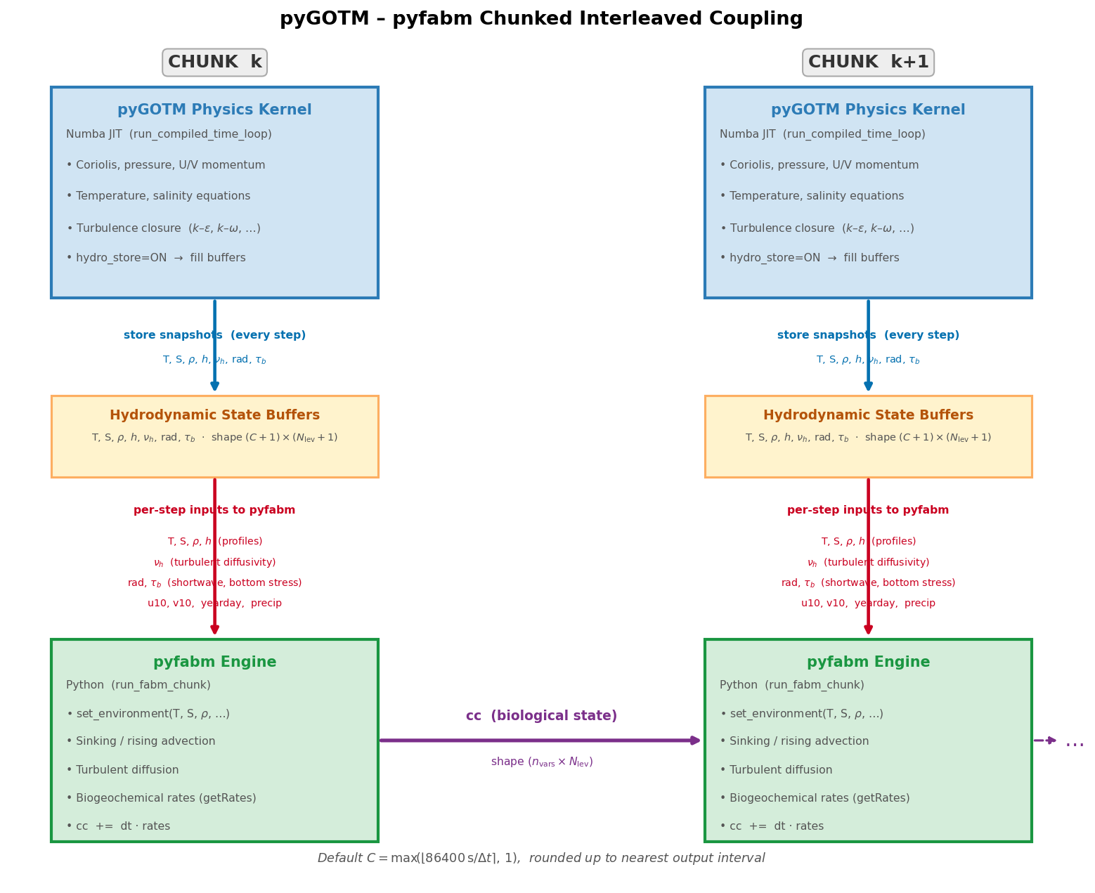
pyGOTM–pyfabm chunked coupling diagram — **Figure** — Chunked interleaved coupling between the pyGOTM Numba physics kernel and the pyfabm biogeochemical engine. Each chunk runs the full physics for \(N_\mathrm{chunk}\) timesteps, stores snapshots of the hydrodynamic state, then drives pyfabm through those same timesteps. Variables exchanged at each step are shown as labelled arrows.¶

Variables Exchanged¶

pyGOTM → pyfabm (dependencies)¶

At every biogeochemical timestep, pyGOTM sets the following FABM dependencies from the stored hydrodynamic snapshots:

FABM dependency name	Shape	Source in pyGOTM
`temperature`	`(nlev,)`	Potential temperature \(\theta\) [°C] — stored snapshot
`practical_salinity`	`(nlev,)`	Practical salinity \(S\) [psu] — stored snapshot
`density`	`(nlev,)`	In-situ density \(\rho\) [kg m⁻³] — stored snapshot
`cell_thickness`	`(nlev,)`	Layer thicknesses \(h_i\) [m] — stored snapshot
`downwelling_photosynthetic_radiative_flux`	`(nlev,)`	PAR profile [W m⁻²] — computed from radiation snapshot, updated after light-feedback
`surface_downwelling_photosynthetic_radiative_flux`	scalar	Surface PAR [W m⁻²] — top-of-column value
`wind_speed`	scalar	Wind speed \(\|\mathbf{u}_{10}\|\) [m s⁻¹] from (u10, v10) forcing
`number_of_days_since_start_of_the_year`	scalar	Fractional day of year (yearday + secondsofday / 86400)
`bottom_stress`	scalar	Bottom friction velocity \(\tau_b\) [Pa] — stored snapshot

Dependencies that are not exposed by the particular FABM model are silently skipped. A call to engine.unresolved_dependencies() reports any required dependencies that have not been set after initialization.

pyfabm → pyGOTM (feedbacks and diagnostics)¶

FABM diagnostic / output	Shape	Effect in pyGOTM
`attenuation_coefficient_of_photosynthetic_radiative_flux` (or `kc`)	`(nlev,)`	Bio-shading: modifies the PAR profile fed back to FABM at the next rates call within the same timestep (light-feedback loop)
Source/sink rates (all state variables)	`(n_vars, nlev)`	Applied to biological concentrations: `cc += dt * rates`
Surface exchange rates	`(n_vars, nlev)`	Added only to the top layer (index `−1`) as air-sea exchange
Bottom exchange rates	`(n_vars, nlev)`	Added only to the bottom layer (index `0`) as sediment flux
Vertical movement velocities	`(n_interior, nlev)`	Sinking or rising advection before the diffusion/reaction step

Within-Chunk FABM Timestep¶

Each biological timestep within a chunk applies the following operations in order, which exactly mirrors the sequence used by gotm_fabm.F90 in the reference Fortran GOTM implementation:

Set environment — copy the stored hydrodynamic snapshots into pyfabm dependencies (temperature, salinity, density, cell thickness, PAR, wind, year-day, bottom stress).
Vertical advection (sinking/rising) — interior state variables with non-zero vertical movement velocities are advected using the conservative P2-PDM scheme (adv_center) with zero-flux boundary conditions at top and bottom. Face velocities are computed by thickness-weighted interpolation of cell-centre velocities to interfaces, replicating lines 1161–1199 of gotm_fabm.F90.
Turbulent diffusion — each interior state variable is diffused vertically using the implicit Crank–Nicolson solver (diff_center) with the turbulent diffusivity \(\nu_h\) from the stored hydrodynamic snapshot. Precipitation dilution is applied as a Neumann surface boundary condition: \(F_\mathrm{surf} = -c_{n,\mathrm{sfc}} \cdot \text{precip}\).
Biogeochemical rates — pyfabm getRates() is called after the transport step so that reaction rates act on the post-transport concentrations. The rates are retrieved three times with different surface/bottom flags to separate bulk, surface, and bottom contributions:
```
bulk_rates  = engine.get_rates(surface=False, bottom=False)
surf_rates  = engine.get_rates(surface=True,  bottom=False)
bot_rates   = engine.get_rates(surface=False, bottom=True)
```
Light feedback — if attenuation_coefficient_of_photosynthetic_radiative_flux is exposed by the model, the PAR profile is recomputed from the biological attenuation and fed back into FABM before a second rates call within the same timestep. This two-pass approach captures the immediate effect of phytoplankton self-shading on the light available for growth.
Apply rates — concentrations are updated:

\[c_i^{n+1} = c_i^n + \Delta t \cdot R_i^\mathrm{bulk} + \Delta t \cdot \delta_{i,\mathrm{top}} \left(R_i^\mathrm{surf} - R_i^\mathrm{bulk}\right)\big|_\mathrm{top} + \Delta t \cdot \delta_{i,\mathrm{bot}} \left(R_i^\mathrm{bot} - R_i^\mathrm{bulk}\right)\big|_\mathrm{bot},\]

where surface and bottom exchange contributions are concentrated in the top and bottom cells respectively. Surface and bottom state variables (e.g. sediment fractions exposed by some FABM models) are updated separately from their single-layer rate arrays.

PAR Profile and Light Feedback¶

The downwelling photosynthetically active radiation (PAR) at cell-centre depth \(z_k\) is computed from the surface radiation snapshot using a two-component exponential attenuation:

\[I_k = I_0 (1 - A) \exp\!\left(-\frac{z_k}{g_2} - K_\mathrm{bio}(z_k)\right),\]

where \(I_0\) is the surface shortwave, \(A\) is the fraction absorbed in the first attenuation component (light_A), \(g_2\) is the background attenuation depth scale (light_g2), and \(K_\mathrm{bio}(z_k) = \sum_{k'=k}^{N} k_{c,k'} \Delta h_{k'}\) is the cumulative biological attenuation integrated downward from the surface using the kc (or attenuation_coefficient_of_photosynthetic_radiative_flux) diagnostic exposed by the FABM model.

When light_g2 ≤ 0, light feedback is disabled and the PAR profile is the stored GOTM radiation profile unchanged.

Memory Layout¶

The hydrodynamic state buffers allocated once per integration are

Array	Shape	Content
`hydro_T`	`(C+1, nlev+1)`	Temperature snapshots (bottom→top, index 0 = initial condition)
`hydro_S`	`(C+1, nlev+1)`	Salinity snapshots
`hydro_rho`	`(C+1, nlev+1)`	Density snapshots
`hydro_h`	`(C+1, nlev+1)`	Cell-thickness snapshots
`hydro_nuh`	`(C+1, nlev+1)`	Turbulent diffusivity snapshots
`hydro_rad`	`(C+1, nlev+1)`	Shortwave radiation snapshots (PAR source)
`hydro_taub`	`(C+1,)`	Bottom stress snapshots (scalar per step)

Row 0 of each buffer holds the state at the start of the chunk (or the initial condition on the first chunk). Rows 1…C hold the state after each physics timestep. The last column (index nlev) is the surface interface value.

If the final chunk is smaller than the default chunk size, the buffers are reallocated to the smaller size so no stale data is used.

FABM NetCDF output buffers are allocated after pyfabm.Model has been instantiated, because only the live model knows its state and diagnostic output names. Memory for those buffers scales as \(O(N_\mathrm{vars} N_\mathrm{out} N_\mathrm{lev})\) for interior variables and \(O(N_\mathrm{vars} N_\mathrm{out})\) for horizontal variables. Physics- only runs allocate no FABM output buffers.