Mean Flow

pyGOTM implements the 1D mean-flow equations from GOTM manual Chapter 3 (Umlauf, Burchard & Bolding).

Momentum Equations

The horizontal momentum equations (Sections 3.2.5–3.2.6) are solved as a coupled system. In the horizontal-mean, incompressible, Boussinesq approximation they read:

\[\frac{\partial U}{\partial t} - fV = - \frac{\partial P_x}{\partial x} + \frac{\partial}{\partial z}\left(\nu_t \frac{\partial U}{\partial z}\right)\]

\[\frac{\partial V}{\partial t} + fU = - \frac{\partial P_y}{\partial y} + \frac{\partial}{\partial z}\left(\nu_t \frac{\partial V}{\partial z}\right)\]

where \(f\) is the Coriolis parameter, \(P_x\), \(P_y\) are the external (barotropic) pressure gradients, and \(\nu_t\) is the turbulent eddy viscosity. Internal (baroclinic) pressure gradients from horizontal density gradients can be included as additional body forces.

The Coriolis term is treated with an exact rotation (Section 3.2.4): the velocity vector \((U, V)\) is rotated by angle \(f \Delta t\) before the momentum diffusion step.

The discretisation uses a Crank–Nicolson scheme (implicitness parameter \(\sigma = 1\)) for the vertical diffusion term, giving an unconditionally stable tridiagonal system solved with the Thomas algorithm at each timestep.

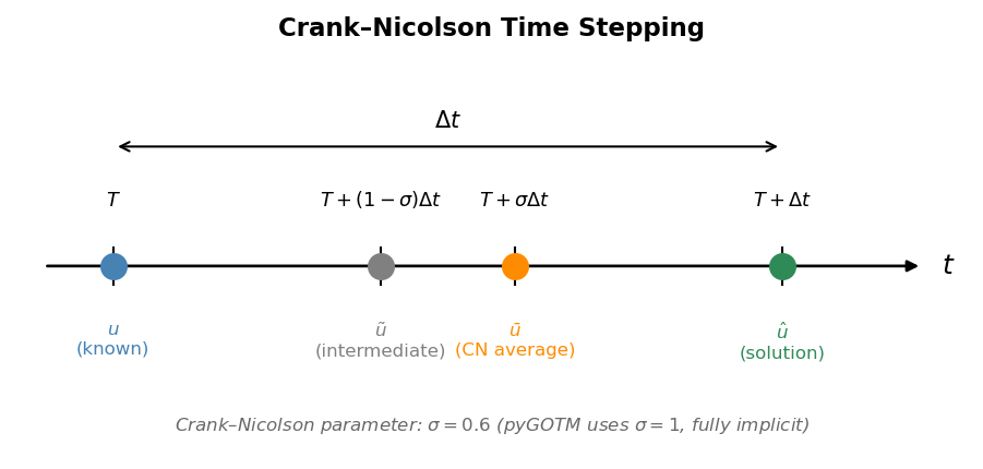
Figure 2 — Crank–Nicolson time stepping. The scheme evaluates the diffusion operator at time \(T + \sigma \Delta t\), a weighted average between the old state \(u\) and the new state \(\hat{u}\). pyGOTM sets \(\sigma = 1\) (fully implicit). (After GOTM manual Fig. 2, p.25.)

Scalar Transport

Both potential temperature \(\theta\) and salinity \(S\) satisfy a general advection–diffusion equation (Sections 3.2.10–3.2.11):

\[\frac{\partial \phi}{\partial t} = \frac{\partial}{\partial z}\left(\kappa_t \frac{\partial \phi}{\partial z}\right) + S_\phi\]

where \(\kappa_t\) is the turbulent scalar diffusivity, and \(S_\phi\) is a source term. For temperature, \(S_\phi\) includes the divergence of the short-wave radiation flux absorbed within the water column.

Boundary conditions at the surface and bottom are of Neumann type (prescribed flux).

Shear Frequency

The squared shear frequency \(M^2\) (Section 3.2.13) is defined as

\[M^2 = \left(\frac{\partial U}{\partial z}\right)^2 + \left(\frac{\partial V}{\partial z}\right)^2 \point\]

It is computed using the energy-conserving discretisation of Burchard (2002), which guarantees that no spurious kinetic energy is generated when converting from mean to turbulent kinetic energy.

Density and Stratification

Density \(\rho\) is computed from \(\theta\) and \(S\) using the UNESCO equation of state (Section 3.2.14, Eq. 39). The squared buoyancy frequency is (Eq. 38):

\[N^2 = -\frac{g}{\rho_0} \frac{\partial \rho}{\partial z} \point\]

\(N^2\) decomposes into thermal and haline contributions (Eqs. 40–42):

\[N^2 = N^2_\Theta + N^2_S \comma\]

where \(N^2_\Theta\) arises from the vertical temperature gradient and \(N^2_S\) from the salinity gradient, each weighted by the corresponding thermal expansion and haline contraction coefficients.

Both \(M^2\) and \(N^2\) are passed to the turbulence closure as forcing.

Bottom and Surface Roughness

The bottom roughness length combines viscous (smooth-wall), form drag (rough wall), and moveable-bed (sediment) contributions (GOTM Eq. 23):

\[z_{0b} = \frac{0.1\nu}{u_{\tau b}} + 0.03 h_{0b} + z_a \comma\]

The bottom friction velocity is (Eq. 24):

\[u_{\tau b} = r\sqrt{U_1^2 + V_1^2} \comma\]

where the drag coefficient \(r\) is (Eq. 25):

\[r = \frac{\kappa}{\ln\!\left(\frac{0.5 h_1 + z_{0b}}{z_{0b}}\right)} \point\]

Charnock’s surface roughness formula (Eq. 26):

\[z_{0s} = \frac{\alpha_c u_{\tau s}^2}{g} \point\]

Staggered Grid

Mean-flow variables (\(U\), \(V\), \(\Theta\), \(S\), \(\rho\)) are carried at cell centres (layers \(i = 1, \ldots, N\)), while turbulent quantities (\(k\), \(\varepsilon\), \(\nu_t\), \(\kappa_t\)) are carried at cell interfaces (\(i = 0, \ldots, N\)). Layer thicknesses \(h_i\) are positive. Index \(i = 0\) is the seabed, index \(i = N\) is the surface.

API Reference

coriolis	Coriolis rotation of horizontal velocity.
friction	Vertical friction and boundary-layer drag.
salinity	Salinity transport equation.
shear	Vertical shear-frequency squared.
temperature	Temperature (potential) transport equation.
uequation	U-momentum (east–west) equation.
vequation	V-momentum (north–south) equation.