Physics Overview
GOTM models a one-dimensional water column — the vertical dimension only. Horizontal gradients of velocity, temperature, and salinity can be prescribed as external forcing, but are not computed. This is appropriate for open-ocean and lake sites where horizontal homogeneity is a reasonable assumption over the simulation period.
Governing Equations
The state vector of a GOTM column consists of:
Horizontal velocity components \(U(z,t)\) and \(V(z,t)\)
Potential temperature \(\theta(z,t)\)
Salinity \(S(z,t)\)
Turbulent kinetic energy \(k(z,t)\) and a second turbulence quantity (\(\varepsilon\), \(\omega\), or a length-scale \(l\))
Each quantity is governed by a 1D transport equation of the generic form
where \(\nu_\phi\) is the appropriate eddy diffusivity and \(S_\phi\) collects all remaining source/sink terms (Coriolis, pressure gradients, radiation, etc.).
Vertical Grid
GOTM uses a staggered finite-difference grid with \(N_\mathrm{lev}\) layers:
Scalar quantities (\(\theta\), \(S\), \(k\), \(\varepsilon\)) are located at layer centres (indices \(1, \dots, N_\mathrm{lev}\)).
Fluxes and diffusivities are located at layer interfaces (indices \(0, \dots, N_\mathrm{lev}\)).
Layer thicknesses \(h_i\) are uniform by default but can be configured.
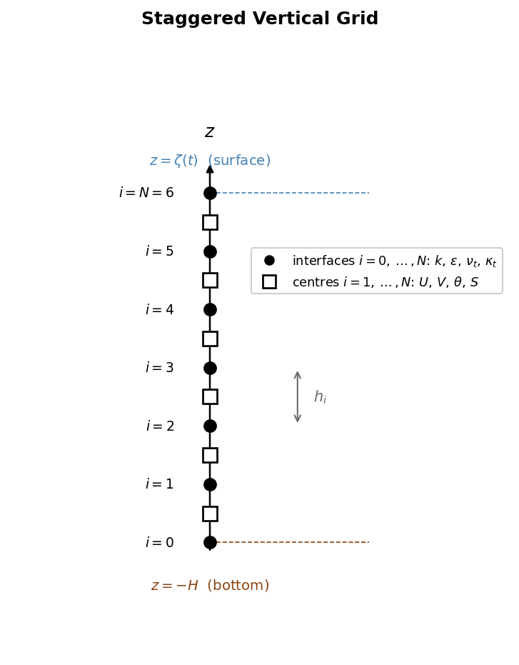
Figure 1 — Staggered vertical grid. Filled circles mark cell interfaces (indices \(i = 0, \dots, N\)) where turbulent quantities (\(k\), \(\varepsilon\), \(\nu_t\), \(\kappa_t\)) are stored. Open squares mark cell centres (indices \(i = 1, \dots, N\)) where mean-flow quantities (\(U\), \(V\), \(\theta\), \(S\)) are stored. Layer thickness \(h_i\) connects adjacent interfaces. (After GOTM manual Fig. 1, p.25.)
Solution Sequence
Each timestep follows this sequence:
Coriolis rotation — rotate \((U,V)\) by angle \(f\Delta t\) (Section 3.2.4).
External pressure gradient — add the depth-uniform barotropic pressure gradient (Section 3.2.7).
Internal pressure gradient — add the baroclinic pressure gradient from the density field (Section 3.2.8).
U/V momentum equations — advance \(U\) and \(V\) with implicit vertical diffusion (Sections 3.2.5–3.2.6).
Ice thermodynamics — update ice cover, thickness, albedo, and transmissivity; diagnose the ocean–ice heat flux that modifies the temperature upper boundary condition (see Ice Thermodynamics).
Temperature equation — advance \(\theta\) including short-wave radiation extinction with the ice-modified albedo and transmissivity (Section 3.2.10).
Salinity equation — advance \(S\) (Section 3.2.11).
Equation of state — update density \(\rho\) and buoyancy frequency \(N^2\).
Shear frequency — compute \(M^2\) from the updated velocity field (Section 3.2.13).
Turbulence closure — advance \(k\) and the second turbulence quantity; update stability functions and diffusivities (Chapter 4).
All section references are to the GOTM manual (Umlauf, Burchard & Bolding).
When FABM biogeochemistry is enabled, the physics loop above runs for a chunk of timesteps (default: ~1 day), storing snapshots of \(T\), \(S\), \(\rho\), \(h\), \(\nu_h\), and radiation. The biogeochemical engine then steps through those snapshots at the same \(\Delta t\). See Biogeochemistry and FABM Coupling for the full description of the coupled loop.
See Also
Mean Flow — mean-flow equation details
Turbulence Closures — turbulence closure details
Air–Sea Interaction — air–sea interaction and boundary conditions
Ice Thermodynamics — ice thermodynamics models (simple through Winton three-layer)
Biogeochemistry and FABM Coupling — pyfabm coupling and chunked biogeochemical loop